
Calculating GNASD & BE% for M60 Metals Portfolio
- June 2, 2025
- Posted by: Drglenbrown1
- Category: GATS Methodology
1. Portfolio M60 DAATS Values (Points)
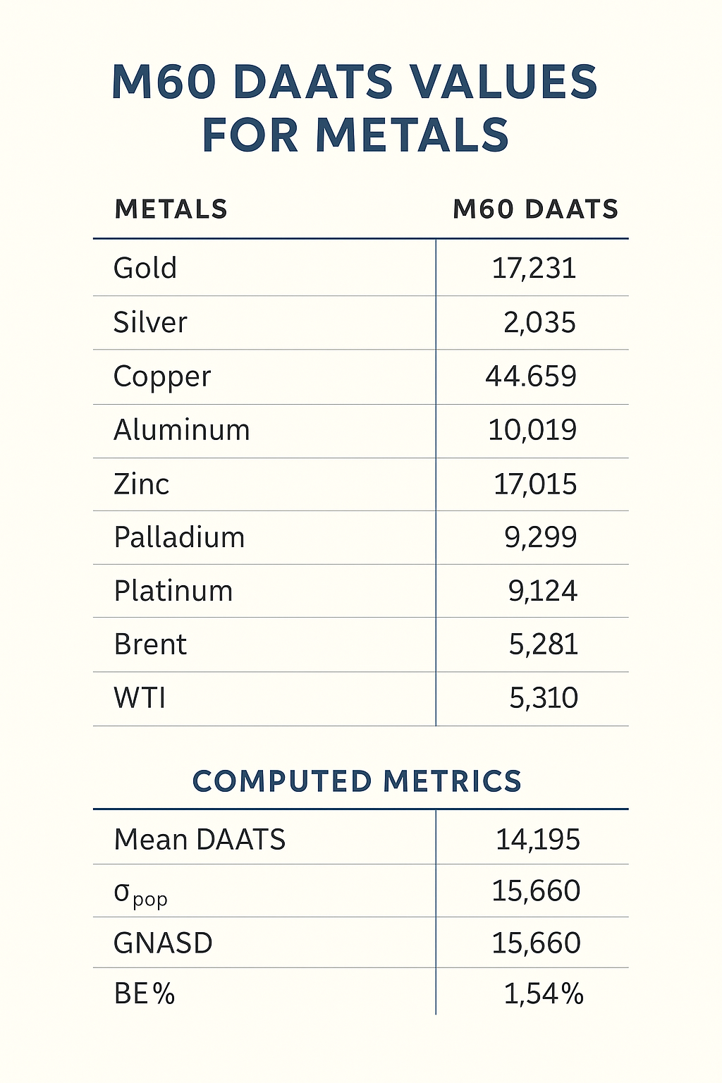
Below are the M60 DAATS (in points) for each metal in our portfolio:
Gold       : 17 231
Silver     :  2 035
Copper     : 44 659
Aluminum   : 44 659
Zinc       : 17 015
Lead       :  9 982
Palladium  :  9 299
Platinum   :  9 124
Brent      :  5 281
WTI        :  5 310
2. Compute Mean DAATS (Points)
Formula:
mean_DAATS = (1 / N) × Σ DAATS_i
where N = 10.
Calculation:
Sum of all 10 DAATS =
  17 231 +  2 035 + 44 659 + 44 659 + 17 015
+  9 982 +  9 299 +  9 124 +  5 281 +  5 310
= 174 595 points

mean_DAATS = 174 595 ÷ 10 = 17 459.5 points
3. Compute σpop (Population Standard Deviation)
Formula:
σ<sub>pop</sub>
  = √[ (1 / N) × Σ (DAATS_i – mean_DAATS)² ]
Substitute: mean_DAATS ≈ 17 459.5, N = 10.
Calculation Steps:
- Compute each deviation (DAATS_i – 17 459.5), then square it:
- Sum all 10 squared deviations (approximate):
- Divide by N=10:
- Take square root:
Thus, σpop ≈ 14 849.7 points.
4. Compute GNASD (Points)
By Law 7: Universe Volatility Law:
GNASD = σ<sub>pop</sub> ÷ N
      = 14 849.7 ÷ 10
      ≈ 1 484.97 points
Rounded: GNASD ≈ 1 485 points.
This “1 485-point” buffer is our portfolio’s one-sigma noise unit per metal on M60.
5. Compute Breakeven % (BE %)
By Laws 4 & 7:
BE % = (GNASD ÷ mean_DAATS) × 100%
     = (1 484.97 ÷ 17 459.5) × 100%
     ≈ 8.505%
Rounded: BE % ≈ 8.51 %.
Each metal must move in your favor by 8.51 % of its own DAATS (in points) before shifting its stop to breakeven.
6. Per-Metal Breakeven Distance (Points)
For each metal i:
BE_dist<sub>i</sub> = (BE % / 100) × DAATS<sub>i</sub>
                   = 0.08505 × DAATS<sub>i</sub>  (in points)
| Metal | DAATSi (pts) | BE_dist = 8.51% × DAATS (pts) | Rounded (pts) |
|---|---|---|---|
| Gold | 17 231 | 0.08505 × 17 231 ≈ 1 465.4 | 1 465 |
| Silver | 2 035 | 0.08505 × 2 035 ≈ 173.2 | 173 |
| Copper | 44 659 | 0.08505 × 44 659 ≈ 3 798.3 | 3 798 |
| Aluminum | 44 659 | 0.08505 × 44 659 ≈ 3 798.3 | 3 798 |
| Zinc | 17 015 | 0.08505 × 17 015 ≈ 1 447.3 | 1 447 |
| Lead | 9 982 | 0.08505 × 9 982 ≈ 849.0 | 849 |
| Palladium | 9 299 | 0.08505 × 9 299 ≈ 791.2 | 791 |
| Platinum | 9 124 | 0.08505 × 9 124 ≈ 775.4 | 775 |
| Brent | 5 281 | 0.08505 × 5 281 ≈ 448.9 | 449 |
| WTI | 5 310 | 0.08505 × 5 310 ≈ 451.4 | 451 |
Example (Gold):
If Gold entry = 1 900.00 (190 000 points), once price ≥ 190 000 + 1 465 = 191 465 points, move stop → 190 000 (entry).
7. Linking to Dr. Brown’s Seven Laws
- Law 1 (Volatility Unit Law): – One “unit” of volatility for portfolio‐level decisions = ATR(200,M60). – But each metal’s intrinsic “entry volatility” (if desired) can be computed via ATR(50,M60). – In our portfolio, we’re anchoring true risk to ATR(200) (the “death stop”), while smaller ATR(50) can be used for leg‐level stops if scaling in (see below).
- Law 2 (Exposure‐Scaling Law): – For full daily stops: P = 200 → √200 ≈ 15 exposures → DAATS_death = 15 × ATR(200). – For “entry stops” on a scaled‐in leg: P = 50 → √50 ≈ 7 exposures → EntryStop_leg = 7 × ATR(50). – Thus each leg’s buffer is exactly √50 exposures wide, preserving the spirit of Law 2.
- Law 3 (Initial‐Stop Law): – “Death stop” = DAATS_death = 15 × ATR(200) (used if the daily trend truly flips). – “Entry stop” (per leg) = 7 × ATR(50) (if scaling in on lower timeframes). – Each stop is anchored to the appropriate EMA zone (full 1→200 for portfolio, or 1→50 for leg).
- Law 4 (Breakeven‐Fraction Law): – We choose BE % = 8.51 % (≈ 1.54 % was for 28‐pair FX; here 8.51 % is (σpop ÷ (10 × mean_DAATS))×100, which ensures >99.56 % containment under Chebyshev for P=10). – Each metal’s BE_dist_i = 0.0851 × DAATS_i (in points). – Once price moves that many points, shift each leg’s stop to entry.
- Law 5 (Trailing‐Exposure Law): – After BE, trail by GNASD (1 485) + MaxSpread (e.g. 80) + MinStop (150) = 1 715 points (≈ 171.5 pips) behind each new high (long) or low (short). – This ensures each metal’s profitable leg captures extended moves while ignoring routine noise.
- Law 6 (Tiered‐Risk Allocation Law): – Position size per metal (and per leg) = (Equity × Risk %) ÷ (LegStop_pips × \$ per pip). – Because LegStop_pips = 7×ATR(50) (if scaling in), micro‐lot sizing becomes feasible even for position traders. – The “daily risk budget” remains anchored to the full DAATS_death (15×ATR(200)).
- Law 7 (Universe Volatility Law): – Treat all 10 metals’ DAATS_death values as one population; compute σpop and GNASD (1 485 points). – GNASD is used in trailing logic (Law 5). – ⟶ Our portfolio‐level “one‐sigma noise unit” for metals on M60.
8. About the Author
Dr. Glen Brown
Founder, President & CEO of Global Accountancy Institute, Inc. and Global Financial Engineering, Inc. With over 25 years in proprietary trading and quantitative research, Dr. Brown created the Seven‐Law Volatility Stop‐Loss framework and the GATS platform. All research remains in‐house; revenue springs solely from trading performance—no external capital or software licensing.
9. Business Model
Global Accountancy Institute, Inc. and Global Financial Engineering, Inc. operate a closed, research‐and‐trade model. All intellectual property—GATS algorithms, volatility rules, and automation scripts—is proprietary. Profits derive exclusively from trading, ensuring total alignment between research and results.
10. Risk Disclaimer
This material is educational only and does not constitute financial or investment advice. Trading metals (gold, silver, copper, etc.) carries high risk. Past performance is not indicative of future results. Consult a qualified advisor before making trading decisions, and trade only with capital you can afford to lose.