Public Doctrine Series
Monetary Engineering
The Better Ways
EMF-2: a monetary framework rebuilt on the levers that survived testing, and the case that it serves households and price stability at once
Dr. Glen Brown · President & CEO, Global Financial Engineering, Inc. and Global Accountancy Institute, Inc.
GFE-PUB-EMF-20261030-A · 30 October 2026
Abstract
The first Engineered Monetary Framework, reported in an earlier internal working paper of the house, beat the strongest conventional interest-rate rule narrowly, and failed three of the six tests I had set for it. Its gains came from a targeted credit instrument and from counting household debt service; its two supply-side devices, a real-time decomposition of inflation and a slow capacity lever, did not work. This paper rebuilds the framework on what survived. EMF-2 keeps the credit instrument and the household term. It reads supply-driven inflation from observed supply prices instead of inferring it after the fact, and it answers that inflation with fast supply relief, measures that act on prices within a quarter, coordinated with the fiscal authority, instead of with an investment that takes two years to add capacity. Alongside the rule, I test the structure of mortgage finance itself.
EMF-2 passes all seven tests I fixed before computing any result, against a stricter standard than its predecessor faced. Out of sample, across fifty-four economies that differ from the central bank’s model, it lowers the conventional loss by 5.5 per cent and the household-weighted loss by 5.2 per cent, cuts debt-service stress above the threshold by two thirds, and controls inflation better, not worse. In a supply shock of the 2021–23 kind it halves the household loss, keeps the peak policy rate more than a point lower, and, where mortgages float, shrinks both the recession and excess home losses by about three quarters. It keeps its advantage when the supply-price signal is as noisy as the shock itself and when the relief is half as potent as assumed. And a structural reform, a cap on how fast a mortgage rate may reset upward, does more for households in a variable-rate economy than any rule change: combined with EMF-2, it makes such an economy as safe for homeowners as one financed by thirty-year fixed loans.
I. Why a second framework
A framework that is merely better than the conventional rule is not the right standard. The right standard is the best design the evidence supports, and the first paper’s value was that it showed, component by component, where the evidence pointed. Three lessons carried over. The policy rate should not have to do everything: a second instrument aimed at credit, rather than at every borrower, produced the whole of the first framework’s average gain. The objective should count what rates do to households with mortgages: the debt-service term halved home losses in a supply crisis. And supply-driven inflation cannot be identified reliably by comparing quarterly surprises in inflation and output, nor answered usefully by investment that takes two years to bear fruit; the first method misread the 2008 oil surge as demand, and the second added demand to an economy already short of supply.
Each of those lessons implies a design. If the central bank cannot infer supply inflation from surprises, it should observe it where it is visible, in energy, food, freight and import prices, which are published daily and monthly and are themselves the channel through which supply shocks reach consumer prices. If capacity investment is too slow to answer a supply shock, the answer must be measures that act on prices within a quarter: releases from strategic reserves, temporary cuts in fuel duty or tariffs, and the clearing of port and logistics bottlenecks. Those are fiscal and administrative instruments, not monetary ones, and the framework treats them as a coordinated arm whose use is triggered by a published rule. And if the policy rate reaches households through their mortgage payments, the speed of that pass-through is itself a design variable, set by the structure of mortgage contracts, and can be governed directly.
II. EMF-2
The economy and the test
The model is unchanged from the first paper. It is a quarterly economy of the Rudebusch and Svensson (1999) family, whose core coefficients are their estimates on United States data, checked against a re-estimate for 1961–2007. Inflation depends on its own past, on the output gap and, through a cost channel, on the real interest rate, since a rate above neutral raises firms’ costs; expectations lean modestly towards the inflation target. Output depends on its own past, on the real interest rate and on a targeted credit instrument, standing in for loan-to-value and debt-to-income limits, that restrains new borrowing at half the potency of a rate rise. Households carry mortgage debt whose effective rate follows the policy rate at a speed set by the share of fixed-rate loans; debt service above 10 per cent of income counts as stress, and a home-loss index rises when that stress coincides with a recession. The policy rate cannot fall below −1 per cent.
Every rule is judged by two quarterly losses. The conventional loss is the squared gap between inflation and its 2 per cent target, plus half the squared output gap, plus a quarter of the squared change in the policy rate. The household-weighted loss adds the squared debt service above the stress threshold and small penalties for using the credit instrument and the relief described below, because neither is free. Rules are tuned on twelve economies and tested on fifty-four, which differ from the central bank’s own model in how strongly expectations are anchored, how hard the interest rate bites, how strong the cost channel is and how steep the Phillips curve is, under shocks the tuning never saw. The benchmark throughout is the best conventional rule: a smoothed rule on inflation and the output gap whose coefficients were optimised on the same economies and shocks, the strongest version of current practice I could construct.
Two elements are new in the rule. A third, the reset cap, belongs to the structure of mortgage contracts and is treated in Section VII.
A supply-price signal
Each quarter the central bank observes z = ε + ν, the supply shock to inflation plus noise. The noise stands for everything that makes a published price index an imperfect reading of supply pressure: measurement error, pass-through that is not one for one, and movements in energy and import prices that are themselves driven by domestic demand. Its standard deviation is 0.5 in the base case and 1.0, as large as the shock itself, in the stress test. The bank runs the signal through its own inflation recursion to estimate how much of current inflation is attributable to supply shocks, and averages the result over four quarters to obtain Ŝ. This replaces the sign method of the first paper, which inferred supply shocks only when inflation and output happened to surprise in opposite directions.
Fast supply relief
The relief instrument f lowers next quarter’s annualised inflation by κ = 0.5 points per unit, adds a small demand impulse of 0.1 per unit because tax and tariff cuts raise spending, is capped at one unit, and carries a penalty of 0.5 per unit squared in the objective because it costs public money. The stress test halves κ. I make no claim that every economy has such tools in the quantity assumed. The claim tested is conditional: if a government can deliver relief of this kind on a published trigger, how much does it help?
The rule
i* = r* + π̄ + f_d (π̄ − π* − Ŝ) + f_s Ŝ + f_y y − f_D max(0, DSR − 10)
m = min(2, k_m · max(0, y)) f = min(1, k_f · max(0, Ŝ))
The policy rate is smoothed with weight ρ on its last value. The credit instrument leans against positive output gaps; the relief answers supply-driven inflation; the rate eases as household debt service rises above the stress threshold. All seven coefficients are optimised on twelve economies, with the same shocks and seeds as the first paper, against the household-weighted objective.
Table 1. Optimised coefficients
| Rule | ρ | Demand infl. f_d | Supply infl. f_s | Output gap f_y | Debt service f_D | Credit k_m | Relief k_f |
|---|---|---|---|---|---|---|---|
| Best conventional (from the first paper) | 0.21 | 0.58 | — | 1.47 | — | — | — |
| EMF-2 | 0.22 | 0.63 | 0.61 | 1.43 | 2.07 | 0.43 | 0.15 |
[Derived] The optimiser again declines to look through supply inflation with the rate: f_s and f_d are almost equal. The supply signal does its work by triggering relief, not by softening the rate. The debt-service response is twice the first framework’s.
III. Seven tests, fixed in advance
Before computing any EMF-2 result I wrote the following conditions to file, with a higher first bar than the original framework faced: a gain of at least 5 per cent on both objectives, not merely a gain.
Table 2. Falsification tests and results
| Test | Requirement | Result | Verdict |
|---|---|---|---|
| F1 Benchmark | Beat the best conventional rule by ≥ 5% on both losses, 54 economies, unseen shocks | Conventional 3.84 vs 4.06 (−5.5%); household 3.89 vs 4.10 (−5.2%) | Passed |
| F2 Inflation | Inflation RMSE no more than 5% worse | 1.41 vs 1.45 (−3.2%) | Passed |
| F3 Noisy signal | Household gain positive with signal noise as large as the shock | 3.98 vs 4.10 (−2.9%) | Passed |
| F4 Weak relief | Household gain positive with relief half as potent | 3.93 vs 4.10 (−4.3%) | Passed |
| F5 Supply case | Beat the conventional rule on household loss, supply episode, variable mortgages | 2.91 vs 5.47 (−47%) | Passed |
| F6 Every part | Removing any component, and re-optimising the rest, raises the household loss | All four removals raise it (Table 6) | Passed |
| F7 Fixed-rate | Do not lose to the conventional rule in the supply episode, long fixed mortgages | 2.57 vs 3.98 (−35%) | Passed |
[Derived] One question could not be tested: whether a priced supply signal would have avoided tightening into the 2008 oil surge. The quarterly United States data used here carry no energy-price series, and recovering the supply shock from the model’s own residuals would assume the answer.
IV. Results
Table 3. Out-of-sample performance, 54 economies, unseen shocks
| Rule | Conventional loss | Household loss | Worst economy (household) | Inflation RMSE | Output gap s.d. | Debt-service excess | Home index | At lower bound |
|---|---|---|---|---|---|---|---|---|
| Taylor (1993), smoothed | 5.40 | 5.44 | 9.81 | 1.68 | 2.10 | 0.043 | 1.56 | 3.2% |
| Best conventional | 4.06 | 4.10 | 6.64 | 1.45 | 1.74 | 0.039 | 1.45 | 6.1% |
| EMF-1 (first framework) | 3.93 | 4.01 | 6.33 | 1.46 | 1.67 | 0.025 | 1.41 | 5.7% |
| EMF-2 | 3.84 | 3.89 | 6.43 | 1.41 | 1.70 | 0.013 | 1.38 | 7.0% |
[Derived] The EMF-1 household loss also penalised its slow capacity lever; the figures are comparable in every other respect. Signal noise 0.5.
EMF-2 improves on the conventional rule on every dimension a household cares about, and on inflation itself. Debt-service stress falls by two thirds, from 0.039 to 0.013. Inflation tracks the target more closely, with an error of 1.41 points against 1.45, because relief removes part of each supply shock before it enters the inflation process. That point answers the most common objection to a framework that weighs household stress, which is that it must buy relief for borrowers with inflation. Here it does the opposite. The cost appears in one column: EMF-2 spends 7.0 per cent of the time at the lower bound against 6.1, because a rate that eases when debt service is high has less room in a downturn. Its worst economy is better than the conventional rule’s but slightly worse than the first framework’s.
Figure 1. Out-of-sample loss relative to the Taylor rule (Taylor = 100)
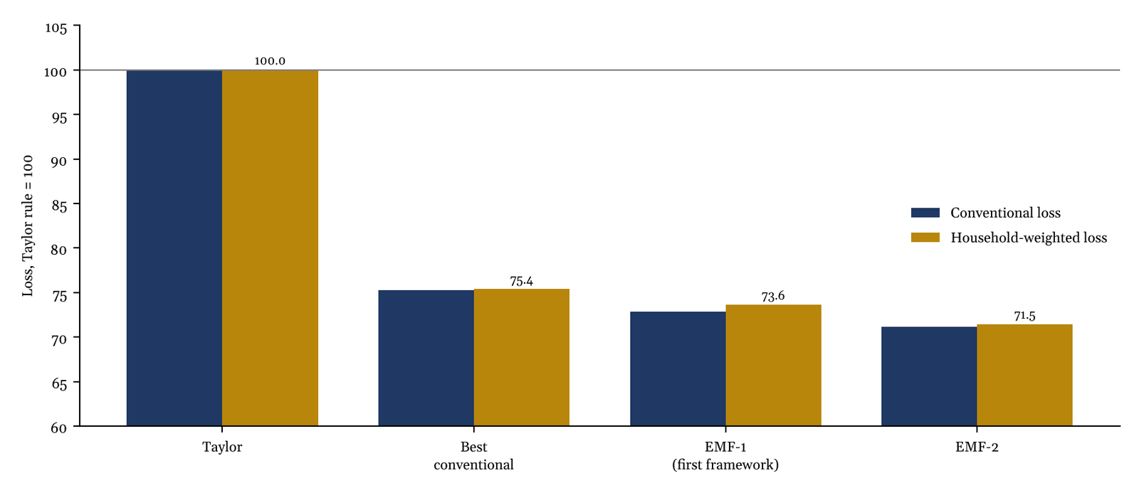
[Derived] Household-weighted losses are labelled. EMF-2 improves on the best conventional rule by more than EMF-1 did, and does so with better inflation control.
Table 4. Stress tests: household loss by signal quality and relief potency
| Condition | Taylor | Best conventional | EMF-2 | EMF-2 vs conventional |
|---|---|---|---|---|
| Perfect supply signal (noise 0) | 5.44 | 4.10 | 3.86 | −6.0% |
| Base case (noise 0.5) | 5.44 | 4.10 | 3.89 | −5.2% |
| Signal as noisy as the shock (noise 1.0) | 5.44 | 4.10 | 3.98 | −2.9% |
| Relief half as potent (κ = 0.25) | 5.44 | 4.10 | 3.93 | −4.3% |
[Derived] The conventional rule uses neither the signal nor the relief, so its figures do not change.
The advantage degrades gracefully. A signal no more informative than the shock it measures still leaves EMF-2 ahead, which matters because the reliability of real-time supply measurement is exactly where the first framework broke.
V. The supply crisis, again
The supply episode is the case for which the framework exists and the one the first version lost. A cost shock of 1.5 points a quarter for six quarters lowers output and is accompanied by a burst of demand stimulus. Results are averaged over two hundred draws of the signal noise.
Table 5. Scripted episodes: household loss, peak policy rate, cumulative output gap, excess home index
| Episode, mortgage regime | Best conventional | EMF-2 | Peak rate (conventional / EMF-2) | Output gap (conventional / EMF-2) | Home excess (conventional / EMF-2) |
|---|---|---|---|---|---|
| Supply, variable (φ 0.75) | 5.47 | 2.91 | 8.9 / 7.8 | −18.9 / −4.7 | 66.0 / 16.9 |
| Supply, long fixed (φ 0.98) | 3.98 | 2.57 | 8.9 / 8.7 | −18.9 / −12.0 | 9.5 / 6.1 |
| Credit boom and bust, variable | 3.91 | 3.01 | 8.3 / 7.0 | −37.1 / −32.5 | 36.8 / 21.4 |
| Credit boom and bust, long fixed | 3.46 | 3.68 | 8.3 / 7.9 | −37.1 / −37.8 | 18.6 / 18.9 |
| Demand overheating, variable | 3.02 | 1.75 | 9.7 / 7.4 | −7.5 / −2.5 | 37.4 / 14.4 |
| Demand overheating, long fixed | 1.38 | 1.15 | 9.7 / 9.2 | −7.5 / −6.6 | 3.8 / 3.3 |
[Derived] The output gap is summed over 40 quarters in point-quarters. The one episode EMF-2 loses, the credit cycle under long fixed-rate mortgages, it loses by 6 per cent.
Under variable-rate mortgages EMF-2 halves the household loss of the supply crisis. The mechanism is visible in Figure 2. Relief, peaking at about 0.55 units, enough to take 0.28 points off annualised inflation in its strongest quarter, lowers the inflation peak from 6.0 to 5.6 per cent and brings inflation back to target sooner than the conventional rule does. With less inflation to fight, the rate peaks at 7.8 per cent instead of 8.9 and falls away quickly. The recession all but disappears, and the home-loss index peaks at about three instead of nearly seven. The same pattern holds in a demand boom, where the credit instrument does the work: the rate peaks more than two points lower and excess home losses fall by three fifths.
The one loss is instructive. In a credit cycle with long fixed-rate mortgages, the household term has little to do, because rates barely reach households, and the credit instrument, tuned on average for a world with more floating debt, leans a little too gently on the boom. The loss is small, and it marks the limit of a single rule set for all mortgage structures; a central bank in a fixed-rate economy would tune the credit gain to its own structure.
Figure 2. Supply crisis under variable-rate mortgages: Taylor, best conventional rule and EMF-2
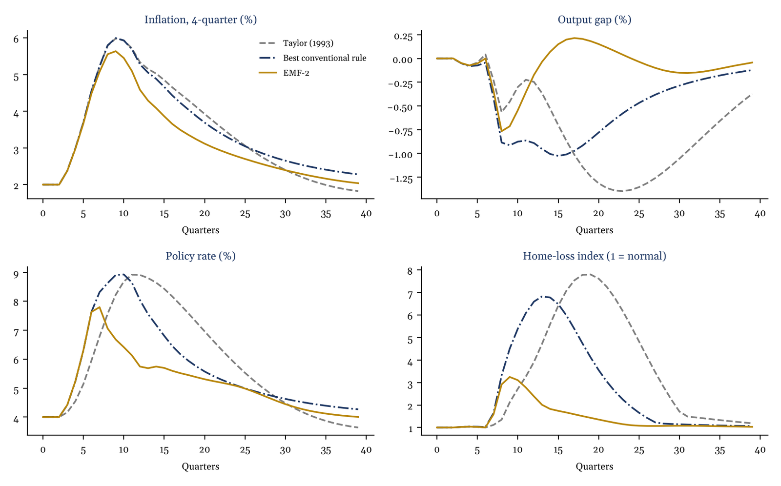
[Derived] EMF-2 (gold) brings inflation down sooner, with a policy rate more than a point lower, an output gap that barely opens and a home-loss index that peaks below half the conventional rule’s.
VI. What each lever does
In the first paper I removed components with the remaining coefficients held fixed. Here I remove each lever and re-optimise everything else, which gives the reduced framework every chance to compensate. A lever earns its place only if the best framework without it is worse.
Table 6. Ablation with re-optimisation
| Variant | Conventional loss | Household loss | Cost of removal (household loss) |
|---|---|---|---|
| EMF-2, full | 3.841 | 3.888 | — |
| Without fast relief | 3.958 | 4.016 | +3.3% |
| Without the supply signal (and so without relief) | 3.957 | 4.015 | +3.3% |
| Without the credit instrument | 3.905 | 3.936 | +1.2% |
| Without the debt-service term | 3.847 | 3.897 | +0.2% |
[Derived] Best conventional rule: 4.064 and 4.102. Each variant is re-optimised from two starts on the training economies and evaluated on all 54.
Fast relief, steered by the supply signal, is now the largest lever, worth 3.3 per cent of household loss on average and most of the gain in a supply crisis. The credit instrument is second. The debt-service term earns little on average, and, as in the first paper, its value is concentrated in the episodes that cost households their homes; it is insurance and should be judged as insurance. The supply signal has no value except through relief: without relief, the optimiser sets the rate’s response to supply and demand inflation equal. That finding, now replicated across both frameworks, is worth stating plainly. In an economy with backward-looking inflation, the policy rate should not look through supply inflation, because that inflation propagates whether or not it is called transitory. The better answer to a supply shock is to act on supply prices directly and leave the rate to do what it does well.
VII. The structure of mortgage finance
The first paper found that the share of fixed-rate mortgages mattered more for home losses than any change in the policy rule. Here I test a lever a government can actually pull in a variable-rate economy without converting its whole mortgage stock: a cap on how fast the effective mortgage rate may reset upward, of one point a year or half a point a year. Such caps exist in parts of the adjustable-rate mortgage market in the United States and have been proposed elsewhere. Downward resets are not capped.
Table 7. Household loss by mortgage structure, base economy, unseen shocks
| Mortgage structure | Best conventional | EMF-2 | Home index (conventional / EMF-2) | Inflation RMSE (conventional / EMF-2) |
|---|---|---|---|---|
| Long fixed, no cap | 4.53 | 4.26 | 1.47 / 1.37 | 1.62 / 1.56 |
| Mixed, no cap | 5.10 | 4.44 | 1.90 / 1.48 | 1.62 / 1.58 |
| Mixed, cap ½ point a year | 4.56 | 4.27 | 1.48 / 1.38 | 1.62 / 1.56 |
| Variable, no cap | 5.82 | 4.64 | 2.11 / 1.55 | 1.62 / 1.60 |
| Variable, cap 1 point a year | 4.74 | 4.35 | 1.62 / 1.42 | 1.62 / 1.57 |
| Variable, cap ½ point a year | 4.52 | 4.26 | 1.43 / 1.37 | 1.62 / 1.56 |
[Derived] The base economy is the central bank’s own model, so losses differ from the 54-economy averages. The caps make no material difference under long fixed-rate mortgages, where resets are already slow.
Two results stand out. Under the conventional rule, a half-point reset cap cuts the household loss of a variable-rate economy by 22 per cent, from 5.82 to 4.52, more than EMF-2 achieves on its own in that economy. And with the cap and EMF-2 together, the variable-rate economy reaches 4.26, matching the 4.26 of a long fixed-rate economy under EMF-2. The framework and the reform are complements: one lowers how high the rate must go, the other limits how fast what remains reaches the household. Together they remove the penalty that variable-rate borrowers otherwise pay for a central bank’s fight against inflation.
A cap is not free, and the model does not count its cost. The interest a capped borrower does not pay in the year of a reset is either deferred, added to the balance or the term, or absorbed by the lender, and a lender that expects to absorb it will price the risk into the mortgage rate or lend less. The test here establishes the size of the household benefit; whether it exceeds the cost to lenders and to credit supply is a question for a model with a banking sector, and I flag it as the first open question of the next paper.
Figure 3. Household loss by mortgage structure
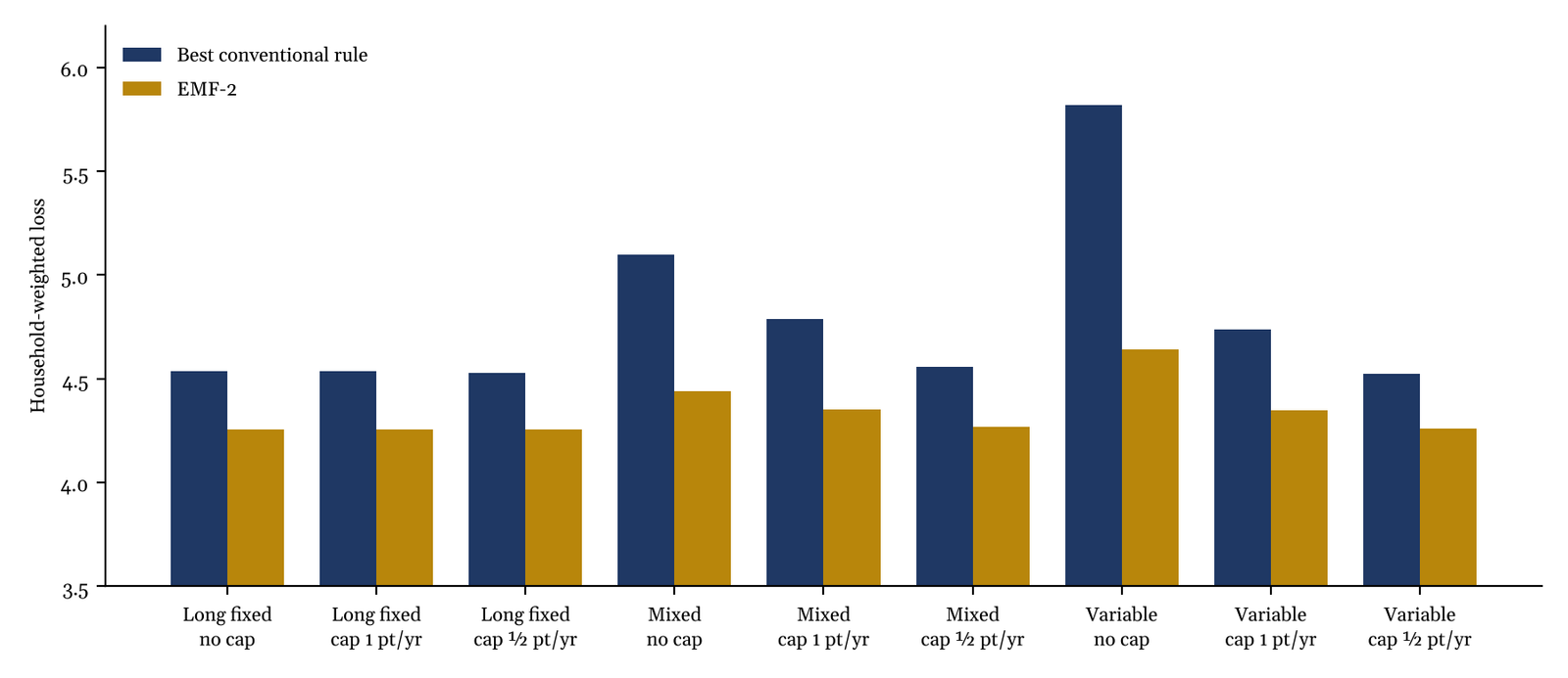
[Derived] The conventional rule’s penalty for variable-rate debt nearly vanishes under a half-point reset cap; EMF-2 with the cap matches EMF-2 under long fixed-rate mortgages.
VIII. The framework as an operating rule
A framework is useful only if it can be run. EMF-2 reduces to six published elements, each governed by a formula from which a committee would have to explain any departure.
| Element | What is published | Who acts |
|---|---|---|
| Policy rate | The rule and its coefficients; the rate the rule prescribes each meeting | Central bank |
| Household stress reading | Aggregate mortgage debt service against a stated threshold, beside inflation | Central bank |
| Supply-price signal | The estimate of supply-driven inflation from energy, food, freight and import prices | Central bank |
| Credit instrument | Loan-to-value and debt-to-income limits that tighten with the output gap by formula | Central bank or macroprudential authority |
| Fast supply relief | A trigger, set by the supply signal, for reserve releases and temporary duty and tariff cuts | Treasury, on the published trigger |
| Mortgage reset cap | A statutory limit on the upward reset of variable-rate mortgages | Legislature, once |
This is a different institution from a committee that sets one rate by discretion. Its decisions are anchored to rules the public can read and check; its departures from them are visible and must be argued for; and the burden of a supply shock is shared between the central bank, which no longer fights it with the rate alone, and the treasury, which holds the instruments that act on supply. [Inference] I believe this is the better design, on the evidence of these two papers, for any economy where a large share of households borrow at rates that reset within a few years.
IX. Limits
The limits of the first paper apply here unchanged. The model is backward-looking, so it cannot show how a credible new framework would itself move expectations. The effect of the real rate on output is borrowed from the literature because the data could not identify it. The cost channel, household block and instruments are calibrated, not estimated, and varied across the robustness set. Four limits are new. The potency of fast relief is an assumption, tested at half strength but not estimated, and its fiscal cost enters the objective only as a penalty. The reset cap’s cost to lenders and to credit supply is not counted. The 2008 test cannot be run without an energy-price series. And the framework still holds the target at 2 per cent: whether a different target or a band would serve households better needs a model in which the level of inflation itself has costs.
Table 8. The seam: principal claims by evidential status
| Claim | Status |
|---|---|
| The 1961–2007 data do not identify the effect of the real rate on output | Witnessed |
| EMF-2 passes all seven tests fixed in advance, including a 5% gain on both losses | Derived |
| EMF-2 controls inflation better than the conventional rule while cutting debt-service stress by two thirds | Derived |
| In a variable-rate supply crisis EMF-2 halves household loss and cuts excess home losses by three quarters | Derived |
| The policy rate should not look through supply inflation; relief should answer it | Derived in two frameworks; inference as policy |
| A half-point reset cap plus EMF-2 makes a variable-rate economy as safe as a fixed-rate one | Derived; lender cost not modelled |
| EMF-2 with a reset cap is the better design for economies with resetting mortgage debt | Inference |
Method note
EMF-2 adds the supply-price signal, fast relief and the reset cap to the model of the first paper; with relief and signal switched off it reproduces that model exactly. EMF-2 is optimised by the Nelder–Mead method from two starts, with up to 600 iterations, on the twelve training economies and one draw of shocks, and evaluated on all fifty-four economies with a fresh draw, two hundred paths of 160 quarters each after a burn-in of forty. Ablations are re-optimised the same way, and the scripted episodes are averaged over two hundred draws of the signal noise. The tests in Table 2 were written down before the run. The best conventional rule’s coefficients are carried unchanged from the first paper, so the benchmark was not re-tuned to suit this comparison.
References
Barth, M. and V. Ramey (2001), “The Cost Channel of Monetary Transmission”, NBER Macroeconomics Annual 16.
Rudebusch, G. and L. Svensson (1999), “Policy Rules for Inflation Targeting”, in J. Taylor (ed.), Monetary Policy Rules, University of Chicago Press.
Shapiro, A. H. (2022), “Decomposing Supply and Demand Driven Inflation”, Federal Reserve Bank of San Francisco Working Paper 2022-18.
Taylor, J. (1993), “Discretion versus Policy Rules in Practice”, Carnegie-Rochester Conference Series on Public Policy 39.
Download the PDF
About the Author
Dr. Glen Brown is President & CEO of Global Financial Engineering, Inc. and Global Accountancy Institute, Inc. He is the architect of the GCPIAUT framework and the broader GATS-native proprietary capital doctrine. His work focuses on sovereign capital governance, algorithmic trading architecture, reserve-first compounding systems, and institutional financial engineering within closed proprietary environments.
Business Model Clarification
Global Financial Engineering, Inc. and Global Accountancy Institute, Inc. operate as closed-loop proprietary institutions. They do not offer public investment products and do not invite retail participation into their proprietary capital architecture. This paper is policy research published for intellectual and institutional discussion.
Disclaimer
This paper is analysis, not advice. It takes no position on any particular decision of any central bank or government, and nothing in it constitutes investment advice, an offer, a solicitation, or a recommendation to buy or sell any financial instrument.